Measurement Systems Analysis (MSA) and in particular Gage R&R studies are tests used to determine the accuracy of measurements. They are the standard way of doing this in manufacturing. Repeated measurements are used to determine variation and bias. Analysis of the measurement results may allow individual components of variation to be quantified. In MSA accuracy is considered to be the combination of trueness (bias) and precision (variation).
This page is the fourth part in a series of pages explaining the science of good measurement. The previous pages included Part 1: Key Principles in Metrology and Measurement Systems Analysis (MSA), Part 2: Uncertainty of Measurement and Part 3: Uncertainty Budgets. The final part is Part 5: Uncertainty Evaluation using MSA Tools. If you’re not familiar with key principles they you’d be best to start at the beginning of this series.
In the previous articles I focused on uncertainty evaluation methods. Uncertainty evaluation may include both experimental variation data (Type A estimates) and other estimates of uncertainties (Type B estimates). A fundamental difference in MSA is that there are no Type B estimates. All of the results come from experimental data. Proponents of MSA would stress that this is a good thing. The results are fully backed by data, there is no room for assumptions which are not supported by evidence. However, there are cases where it may be important to consider uncertainties which are not (or cannot be) observed experimentally, as we will see later in the article.
Type 1 Gage Study
The most fundamental MSA experiment is the Type 1 Gage Study. This involves measuring a single calibrated reference part a number of times, ideally 50 or more. The mean of all the measurement results, minus the reference part’s calibrated value, is the bias. The standard deviation of all the measurement results is the precision. If the bias is small compared to the standard deviation then there may not actually be any bias at all. Due to random variations we will see some small bias which will be different each time with repeat the study.
The amount by which the bias will randomly change with each study is given by the Standard Error in the Mean, this is found by dividing the standard deviation by the square root of the number of repeat measurements (n) in the study:
Generally a normal distribution is assumed. If the bias is equal to the standard error then there is about a 67% chance that there is no bias at all and what we are seeing is simply a result of the random variation in the measurement system. Typically a significance test at 5% is used to determine whether the bias is statistically significant. Therefore we would consider the bias significant if it is greater than 2 x SE.
If we know the tolerance of the part to be measured then we can also consider if the variation is a significant percentage of this tolerance. This is a way of deciding if the measurement is capable of correctly identifying which parts conform to the tolerance specification. Clearly if the measurement variation is larger than the tolerance then even if the parts are all perfect they will frequently be randomly failed due to variation in the measurement results. Different rules of thumb are often used to decide whether a measurement is capable. Often a measurement is regarded as capable if the variation is less than 10% or 20% of the tolerance. Sometimes measurement capability is evaluated using Cg and Cgk. Cg ignores the bias in the measurements and can be considered the potential capability if the bias is corrected. It is given by
where K is some percentage of the tolerance, often 20%, Tol is the process tolerance, L is a number of standard deviations thought to represent the actual or target process spread and σ is the standard deviation in the measurement results.
It should be clear that K and L are just arbitrary numbers added into the equation. For this reason I prefer not to use Cg. I believe it is more intuitive and useful to simply state the standard deviation as a percentage of the tolerance. To do this you simply divide the standard deviation by the tolerance.
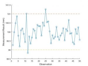
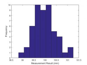
A run chart and a histogram are often plotted for the measurements in a Type 1 Gage Study. These are ways of checking that the results appear to show random and normally distributed variation.

A run chart is simply a plot of each measurement in the order in which it was carried out. It gives a good indication of whether the variation is random. If there is some trend or pattern this would indicate that the variation is not random.

A histogram gives an indication of the underlying probability distribution. It is often assumed that this is a normal distribution. Don’t expect to see a clear bell shaped curve unless the sample has many hundreds of measurements but it should be roughly the right shape.
Gage R&R Study – the standard Measurement Systems Analysis tool
A Gage Repeatability and Reproducibility or Gage R&R study gives a bit more information about a measurement process. Typically a crossed study would be carried out in which 3 operators each measure 10 parts 3 times. There should be at least 10 parts chosen to represent the actual or expected part-to-part variation in the process. The parts should be taken at different times, on different shifts and from different machines or lines. Each measurement result is recorded along with the part which was measured and the operator who measured it.
An Analysis of Variance (ANOVA) is then carried out. This is similar to the calculation of standard deviation but more complicated. When calculating standard deviation you first find the mean, then the difference between each value and the mean, the standard deviation is effectively the average of these differences. In ANOVA you consider each factor effecting the variation, in this case there is variation due to variation in the true values of the parts, due to the measurement system and due to the operator making the measurement. Therefore many different means are calculated for sub-sets of the measurements having the same operator and the same part. Differences are calculated between individual measurements and these mean by part and mean by operator values. In this way variation due to each factor can be identified. The actual maths is fairly involved but if you want to understand it then my article on calculating Gage R&R in Excel is a good place to start.
When Measurement Systems Analysis might not detect uncertainty
In the introduction I mentioned a fundamental difference between MSA and uncertainty evaluation. In MSA all of the results come from experimental data, there is no way of including an uncertainty we have obtained in some other way (Type-B uncertainty) such as from a calibration certificate. Proponents of MSA would stress that this is a good thing. The results are fully backed by data, there is no room for assumptions which are not supported by evidence. However, there are cases where it may be important to consider uncertainties which are not (or cannot be) observed experimentally. Let’s consider some examples of this.
The simplest example is that of a calibration uncertainty. Consider when a gage study is used to determine the bias of an instrument. The experimental data shows the difference between the mean of the measurement results and the calibrated value for the reference part. It does not give the bias from the true value of the reference part. Due to uncertainty in the calibration of the reference part it is possible that the reference part may be significantly larger than its calibrated value. We may therefore not detect a bias in our instrument.
MSA deals with this issue by stipulating that the calibration uncertainty should be less than 10% of the instrument’s standard deviation. This results in the calibration uncertainty having a negligible contribution to the uncertainty of the instrument. However, if it is not possible to obtain a reference part with such a small relative uncertainty then there is no way of accounting for its contribution.
MSA’s exclusive use of experimental data is more problematic where many systematic effects may be present. Even if we only consider the effect of thermal expansion on a part it is often difficult to experimentally quantify the effects. To do so we would need to ensure that a gage R&R study was carried out over a period of time representing the full thermal variation and using reference parts which represent the full range of possible coefficients of thermal expansion (CTE). But the CTE of parts is likely to change suddenly with a change in batch of raw materials, designing an experiment to replicate this effect is unlikely to be practical.
If an MSA experiment is designed to consider every influence quantity then this becomes very similar to an uncertainty evaluation. The key different is that in uncertainty evaluation there are Type B uncertainties to allow for the fact that it is impractical to vary every influence and account for it statistically.
In practice Gage R&R studies are normally simple standardized studies which do not consider all systematic effects. They are a good check, the total Gage R&R should never be greater than the combined uncertainty – or this is an indication that the uncertainty evaluation is incorrect. Gage R&R is also a valuable way of determining Type A uncertainties for inclusion in an uncertainty budget. In the final part of this series I explain how to carry out uncertainty evaluation using MSA tools.