Evaluating Uncertainty of Measurement

This page is the second part of a series of pages explaining the science of good measurement. In Part 1: Key Principles in Metrology and Measurement Systems Analysis (MSA) concepts such as uncertainty of measurement, confidence and traceability were introduced. This page goes into greater depth about uncertainty of measurement introducing types of uncertainty was well as some basic statistics used in uncertainty evaluation. It is followed by Part 3: Uncertainty Budgets, Part 4: MSA and Gage R&R, and Part 5: Uncertainty Evaluation using MSA Tools.

All measurements have uncertainty which arises from many sources such as repeatability, calibration and environment. Calculating the total uncertainty resulting from all sources involves first estimating the contribution from each source and then determining how these will combine to give a combined standard uncertainty.

Type A and Type B Sources of Uncertainty

Sources of uncertainty are classified as Type A if they are estimated by statistical analysis of repeated measurements or Type B if they are estimated using any other available information. For example to find the repeatability of an instrument we could simply measure the same quantity 20 times and analyse the different results we got, this would be a Type A uncertainty. To find the uncertainty in our calibration reference standard by this method would be impractical, for this we simply look up the uncertainty on it’s calibration certificate, this is a Type B uncertainty.

Basic Statistics required for Uncertainty Evaluation

In order to give values for the uncertainties an understanding of basic statistics is required; standard deviations, probability distributions such as the normal distribution and the central limit theorem. These are explained below.

Standard Deviation

In order to find the repeatability of an instrument we might measure the same quantity 20 times. We will then have 20 slightly different measurement results which give an idea of how much the instrument varies when measuring the same thing, we need to find a number which represents this variation. The simplest number to find would be the range in the data; the biggest value minus the smallest value, but this wouldn’t really represent the spread of all the measurements very well and the more measurements we made the bigger it would get which suggests it is not a reliable method. The standard deviation is a number which can be calculated which is essentially the mean average of how far each individual measurement is from the mean average of all measurements. This is best understood with an example….

The standard measure of uncertainty is the standard deviation so one ‘standard uncertainty‘ means one standard deviation in the measurement.

Probability Distributions and the Central Limit Theorem

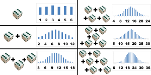
I’m going to explain what a probability distribution is by asking you to imagine rolling some dice. First just roll one dice. You can roll a 1, 2, 3, 4, 5 or 6, and you have an equal chance of rolling any one of them. If you roll the dice 100 times and plot a bar graph of the score against the frequency (the number of times you got that score) then you will end up with 6 bars all of equal height. These bars form a rectangular shape and this is known as a rectangular distribution; the result can be any value between some limits. Uncertainty due to rounding to the nearest increment on an instrument’s scale has a rectangular distribution.

Now consider rolling 2 dice; A and B. you can score anywhere between 2 and 12. But now there is not an equal chance of getting any score. There is only one way to score 2 (A=1 and B=1), there are two ways to score 3 (A=1 and B=2, A=2 and B=1) and so on. The chances keep increasing until you get to a score of 7, which can arise from six different permutations of dice, and then the odds decrease until we get to a score of 12 for which there is again only one way to roll it; both dice must be sixes. If we plot these scores on a bar chart we get a triangular distribution. This is interesting because it doesn’t only apply to dice, if we combine the effects of any two random events with rectangular distributions or similar magnitude then we get a triangular distribution.

If we add more dice things get even more interesting. The peak of the triangle starts to flatten and the ends start to trail off to form a bell shape known as the normal distribution. In fact the central limit theorem states that a number of independent distributions of any shape will combine to give a normal distribution. Combined uncertainty can therefore generally assumed to be normally distributed even when many of the components of uncertainty are not. This is useful as if we know our uncertainty is normally distributed then we know what the probability is of a measurement being in error by more than one standard uncertainty (68%), by more than two standard uncertainties (95%) etc

The Central Limit Theorem – One Die Gives and Equal Chance of a Number Between 1 and 6 but the Sum of 2 Dice is a Triangular Distribution between 2 and 12. More Dice tend towards a Normal Distribution

Some typical sources of uncertainty

Uncertainty of measurement can arise from many sources. I tend to focus on dimensional measurements but the principles of uncertainty evaluation and many of the sources of uncertainty can be applied to any measurement for example time, temperature, mass etc. Some sources of uncertainty which found in all virtually all traceable measurements are the uncertainty of the reference standard used for calibration, the repeatability of the calibration process and the repeatability of the actual measurement. Environmental uncertainties such as the temperature will be significant sources of uncertainty for many measurements. Resolution or rounding may not be a significant source of uncertainty for digital instruments reading out to many decimal places beyond the repeatability of the system but is often significant for instruments with a manually read scale such as rulers, dial gauges etc. Alignment is often a major source of uncertainty for dimensional measurements.

Alignment Errors

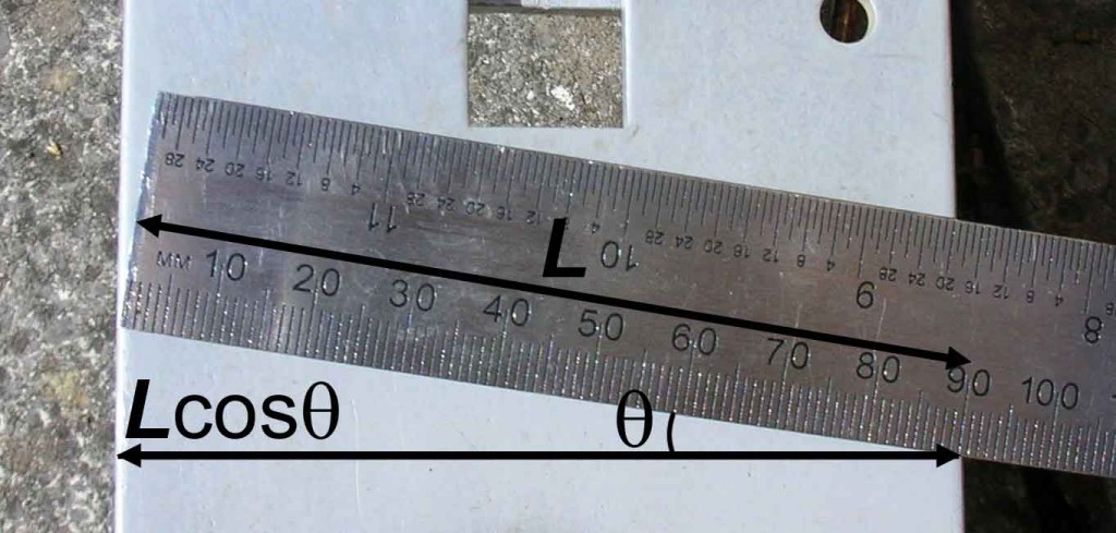
Alignment is a common source of uncertainty in dimensional measurement. For example when a measurement of the distance between two parallel surfaces is made it should be perpendicular to the surfaces. Any angular deviation from the perpendicular measurement path will result in a cosine error in which the actual distance is the measured distance multiplied by the cosine of the angular deviation.

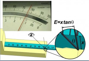
Cosine Error, Common Source of Uncertainty of Measurement — Cosine Error is a Common Source of Uncertainty of Measurement

Another common alignment error is parallax error. This results from viewing a marker, which is separated by some distance from the scale or object being measured, at an incorrect angle. Parallax error commonly observed when a passenger in a car reads the speedometer. Another common example is when the markings on the upper surface of a ruler are used to measure between edges on a surface. If the viewing angle is not perpendicular to the ruler this will result in parallax error.

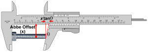
Parallax error is commonly observed when a passenger in a car reads the speedometer or when using a ruler with the markings on the upper surface

Abbe Error is similar to parallax error but rather than resulting from alignment of viewing angles it results from alignment of machine axes. The distance between the axis along which an object is being measured and the axis of the instruments measurement scale is known as the Abbe Offset. If the distance along the object is not transferred to the distance along the scale in a direction perpendicular to the scale then this will result in an error. The size of this error will be the tangent of the angular error multiplied by the Abbe Offset. Instruments such as Vernier callipers are susceptible to Abbe Error as the measurement scale is not co-axial with the object being measured. Micrometers are not susceptible to Abbe Error.

Calipers are susceptible to Abbe Error since the Measurement Scale is not Co-Axial with the Axis of Measurement — An Instrument is Susceptible to Abbe Error if the Measurement Scale is not Co-Axial with the Axis of Measurement

Repeatability and Reproducibility

Repeatability is estimated by making a series of measurements, generally by the same person and under the same conditions, and then finding the standard deviation of these measurements. Reproducibility is estimated by making a series of measurements, each by a different person.

One challenge in evaluating uncertainty of measurement is determining which sources of uncertainty contribute to the observed repeatability. For example it may be that alignment errors vary randomly, contributing to repeatability, and therefore do not need to be evaluated as a separate component of uncertainty. Experience and judgement often play a role in such evaluations.

One method of establishing both repeatability and reproducibility in a single test is a ‘Gage Repeatability and Reproducibility (Gage R&R) Analysis of Variance (ANOVA)’. Using this method several different parts are measured by a number of different people but each part is usually only measured 2 or 3 times by each person. The order of the parts is randomized. The ANOVA statistical analysis is then used to separate out the variation in the results which is due to three sources; the actual component variation; the repeatability of the measurement system; and the reproducibility of results between different people. Gage R&R is a very good way to establish the repeatability and reproducibility components of measurement uncertainty but effort spent on this should not be seen as a substitute for evaluating other sources of uncertainty such as calibration and environment.

Resolution

Uncertainty of measurement due to resolution is a result of rounding errors. For many digital instruments the readout resolution is many times smaller than the actual instrument uncertainty. In such cases rounding errors due the instrument resolution are insignificant.

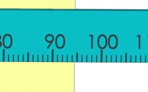
For more traditional instruments resolution is often a significant source of uncertainty. The maximum possible error due to rounding is half of the resolution. For example when measuring with a ruler which has a resolution of 1 mm the rounding error will be +/- 0.5 mm which has a rectangular distribution. Converting a tolerance with a rectangular distribution into a standard uncertainty is covered later.

Rounding Errors Can be up to Half of the Resolution of an Instrument

Temperature

Temperature variations effect measurements in a number of ways:-

Thermal expansion of the object being measured and of the instrument used to measure it
For interferometric measurements changes in the refractive index
For optical measurements which depend on light following a straight line path temperature gradients will cause refraction leading to bending of the light and therefore distortions

Calibration

Any errors in the reference standard used to calibrate a measurement instrument are transferred during calibration. Instruments therefore inherit uncertainty from their calibration standard. The actual process of calibration is also not perfectly repeatable; therefore additional uncertainty is introduced through the calibration process.

If calibration has been carried out by an accredited calibration lab then an uncertainty will be given on the calibration certificate. This is not the uncertainty for measurements made using the instrument; it is simply the component of uncertainty due to calibration. This point is often overlooked.

When carrying out a calibration a complete uncertainty evaluation must be carried out for the calibration process. The combined uncertainty for the calibration then becomes a component of uncertainty for measurements taken using the instrument.

Combining individual sources of Uncertainty of Measurement

Once the individual sources for the uncertainty of a measurement have been identified and quantified a combined uncertainty should be calculated. This is the actual uncertainty of measurement for the process being considered.

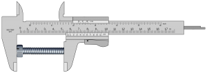
As an introduction to the process of combining uncertainty we will first assume that all sources are normally distributed. Considering the measurement of a bolt, let’s assume that there are just two sources of uncertainty, the thermal expansion of the bolt and the uncertainty of the calliper measurement itself. The measurement result (y) will therefore be given by

y=X+Δx_T+Δx_C
where x is the true length, Δx_T is the error due to thermal expansion and Δx_C is the error due to the calliper measurement itself.

A Simple Example of Combining Uncertainty for the Measurement of a Bolt using Callipers

The error due to each source is not known; each error source has an uncertainty which defines the range of values which we might expect it to take. The probability that both errors will be maximal or minimal at the same time is very small. Therefore to simply add up the uncertainties would be overly pessimistic. Instead the component uncertainties are combined statistically to give a combined uncertainty.

The measurement result is given by y=f(x) where x1, x2 etc are inputs such as the true length and the various errors. Each input has an associated uncertainty u(xi). The combined uncertainty is then given by:-

$U_{c} ^{} \left(y\right)=\sqrt{\sum _{i=1}^{N}\left[\frac{\partial f}{\partial x_{i} } \right]^{2} u^{2} \left(x_{i} \right) }$

For simple cases, such as our example of the callipers measuring the bolt, where
y = x₁ + x₂2 … x_n
The partial derivatives will all be equal to one so that

$\begin{array}{l} {\frac{\partial f}{\partial x_{i} } =1\quad \Rightarrow } \\ {U_{c} ^{} \left(y\right)=\sqrt{\sum _{i=1}^{N}\left[\frac{\partial f}{\partial x_{i} } \right]^{2} u^{2} \left(x_{i} \right) } =\sqrt{\sum _{i=1}^{N}u^{2} \left(x_{i} \right) } } \end{array}$

Applying this to the example

y=X+Δx_T+Δx_C

The true length (X) has no uncertainty, leaving two sources of uncertainty; the uncertainty in the error due to thermal expansion u(Δx_T); and the uncertainty in the error due to the calliper measurement itself u(Δx_C). The combined uncertainty is therefore simply

$U_{c} ^{} \left(y\right)=\sqrt{u^{2} \left(\Delta x_{T} \right)+u^{2} \left(\Delta x_{C} \right)}$

This information can be used to create a simple uncertainty budget. First the standard uncertainty for each source of uncertainty is estimated.

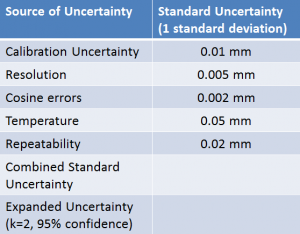
A table listing the standard uncertainty for each source of uncertainty of measurement — In this simple uncertainty budget for a calliper measurement each source of uncertainty is first estimated

There is a simple functional relationship where the errors are simply added to the true value to give the measurement result. The combined uncertainty is therefore simply the square root of the sum of each component uncertainty squared (RSS). The combined uncertainty is multiplied by a coverage factor to give the uncertainty at a required confidence level (the expanded uncertainty).

The simple uncertainty budget is completed by calculating the combined standard uncertainty and expanded uncertainty

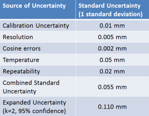
The example on this page was a simplification to introduce the concepts. An example of a proper uncertainty budget is given in the next section.

Part 3: Calculating an Uncertainty Budget…